卷积神经网络(CNN)识别手写数字MNIST(附代码)

写在前面

1. 此文是我学习AI入门的笔记。学习教材《neural networks and deep learning》，作者Michael Nielsen。
2. 这是一本免费的书籍，网址在这里。
3. 此文是第六章内容的学习总结，前几章的内容总结可以见我的博客。
4. 初学者入门，如有错误，请指正。

简介卷积神经网络

在之前的学习中，我们都是使用全连接的神经网络来处理问题的。即，⽹络中的神经元与相邻的层上的每个神经元均连接，在此之前我们已经获得了98%的分辨率了。

但是在识别手写数字的问题上，这样连接方式有很大的缺点：

它忽略了图像本身的空间结构（spatial structure），而以同样的方式对待所有的输入像素。

今天介绍的卷积神经网络则可以很好的利用图像的空间结构，是处理图像分类问题的一个很好的框架。

学习CNN框架，就要了解它的三个基本概念：

• Local receptive fields 局部感受野
• shared weights 共享权重
• pooling 池化

1. 局部感受野

在识别手写数字的问题中，输入层是28 * 28的图像的像素灰度，因此输入层共有28 * 28=784个神经元。

在CNN中，我们将这784个神经元看做方形排列。

当我们把输入层神经元连接到隐藏神经元层时，我们不会全部映射，而是进行小的、局部的连接。

例如，我们将输入层一个5 * 5的方形区域连接到隐藏层的一个神经元。

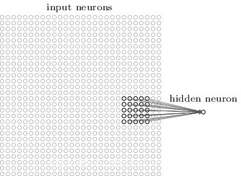
这个输⼊图像的区域被称为隐藏神经元的局部感受野。它是输入像素上的一个小窗口。每个连接学习⼀个权重。而隐藏神经元同时也学习⼀个总的偏置。你可以把这个特定的隐藏神经元看作是在学习分析它的局部感受野。

然后我们在输入层上移动局部感受野，而每一个不同的局部感受野对应了隐藏层上的一个神经元。

例如，输入层左上角的25个神经元对应第一个隐藏神经元。

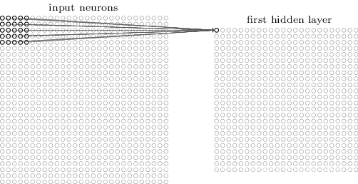
然后我们向右移动一个像素（神经元），对应隐藏层第二个神经元。

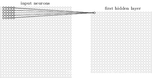
如此不断移动，我们会得到一个24 * 24个神经元的隐藏层。

当然我们也可以使用不同的跨距（stride length），比如一次移动两个像素。在此处我们取跨距为1。

2. 共享权重和偏置

对于每一个隐藏层神经元，它具有一个偏置，并连接了一个5 * 5的局部感受野，所以也有5 * 5个权重。

对于同一层的每一个隐藏神经元，我们使用相同的偏置和5* 5权重，换句话说，对于隐藏层的每一个神经元，其输出公式为

• σ是神经元的激活函数，可以是我们之前学习过的S型函数。
• b是共享偏置
• w~l,m~是一个共享的5 * 5 的权值数组
• a~x,y~表示位于x，y位置的输入激活值

对同一个隐藏层使用相同的权重和偏置，就可以让此层的神经元在图像的不同位置学习一个特定的特征。

也因此，我们将从输入层到隐藏层的映射称为特征映射（feature map）
将定义特征映射的权重和偏置称为共享权重（shared weights）和共享偏置（shared bias），也称作卷积核（kernel）或滤波器（filter），这是一些文献中可能会使用的术语。

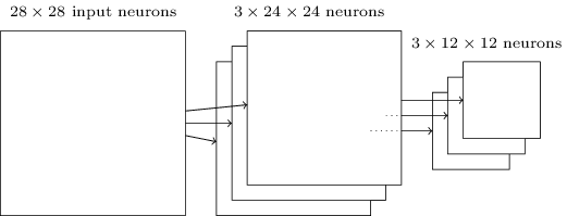
⽬前我描述的⽹络结构只能检测⼀种局部特征的类型。为了完成图像识别我们需要超过⼀个的特征映射。所以⼀个完整的卷积层由几个不同的特征映射组成：

在上图所示的例子中，我们使用了三个特征映射，每个特征映射由一个5 * 5的权值数组和一个偏置，可以探测图像的一个特征。

而在下面我们的实际开发案例中，我们使用了20个特征映射（卷积核、滤波器），学习了下面的20种图形特征。


每个映射有⼀幅 5 × 5 块的图像表示，对应于局部感受野中的 5 × 5 权重。白色块意味着⼀个小（更小的负数）权重，所以这样的特征映射对相应的输⼊像素有更小的响应。更暗的块意味着⼀个更⼤的权重，所以这样的特征映射对相应的输⼊像素有更大的响应。

共享权重和偏置的⼀个很⼤的优点是，它⼤⼤减少了参与的卷积网络的参数。对于每个特征映射我们需要 25 = 5 × 5 个共享权重，加上⼀个共享偏置。所以每个特征映射需要 26 个参数。如果我们有 20 个特征映射，那么总共有 20 × 26 = 520 个参数来定义卷积层。

作为对比，假设我们有⼀个全连接的第⼀层，具有 784 = 28 × 28 个输⼊神经元，和⼀个相对适中的 30 个隐藏神经元，正如我们在本书之前的很多例⼦中使⽤的。总共有 784 × 30 个权重，加上额外的 30 个偏置，共有 23, 550 个参数。换句话说，这个全连接的层有多达 40 倍于卷基层的参数。

3. 池化

卷积神经网络除了卷积层之外，还有池化层。池化层通常在卷积层之后，主要作用是简化从卷积层输出的信息。

最大值池化（max-pooling）

最大值混合是一个常见的池化方式。一个池化单元将卷积层一个区域（例如2
*2）中的最大激活值作为其输出：

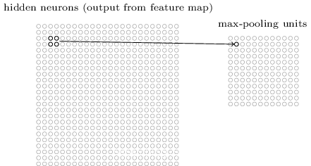
注意既然从卷积层有 24 × 24 个神经元输出，混合后我们得到 12 × 12 个神经元。

正如上⾯提到的，卷积层通常包含超过⼀个特征映射。我们将最⼤值混合分别应⽤于每⼀个特征映射。所以如果有三个特征映射，组合在⼀起的卷积层和最⼤值混合层看起来像这样：

通过池化的方式，网络可以得知，对于给定的一种图形特征，它大致分布在图像的哪些位置，而不需要处理大量具体的位置信息，这有助于减少在后面的层中所需的参数的数目。

L2池化（L2-pooling）

L2-池化则是取 2×2 区域中激活值的平方和的平方根。

虽然细节不同，但是两种池化方式都被广泛应用到实际中。

综合

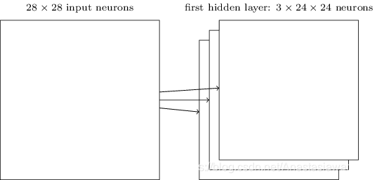
我们现在可以把这些思想都放在⼀起来构建⼀个完整的卷积神经⽹络。它和我们刚看到的架构相似，但是有额外的⼀层 10 个输出神经元，对应于 10 个可能的 MNIST 数字（’0’，’1’，’2’ 等）：

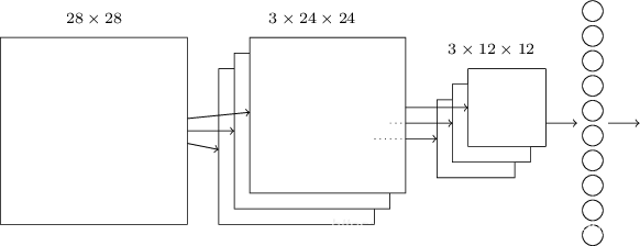
这个⽹络从 28 × 28 个输⼊神经元开始，这些神经元⽤于对 MNIST 图像的像素强度进⾏编码。

接着的是⼀个卷积层，使⽤⼀个 5×5 局部感受野和 3 个特征映射。其结果是⼀个 3×24×24隐藏特征神经元层。下⼀步是⼀个最大值池化层，应⽤于 2 × 2 区域，遍及 3 个特征映射。结果是⼀个 3 × 12 × 12 隐藏特征神经元层。

网络中最后连接的层是⼀个全连接层。更确切地说，这⼀层将最⼤值混合层的每⼀个神经元连接到每⼀个输出神经元。这个全连接结构和我们之前章节中使用的相同。

代码

现在将卷积神经网络应用于手写数字MNIST问题。

环境配置

此处提供代码的Github下载地址，我们此次运行的代码是network3.py,是之前运行的network.py和network2.py的加强版。

跟前面的章节相似，我们会使用Anaconda来运行作者的python2 的代码，同时需要numpy库和Theano库。

Anaconda和numpy库的下载及使用可以参考我之前的一篇博客：使用神经网络实现手写数字识别（MNIST）

我们还需要下载Theano库来运行代码。网上关于Theano的下载和安装教程不多，但是我基本都没怎么看懂（咳咳）。自己倒腾了一下不知道为啥就可以运行了（那就这样吧），此处放上Theano的官方文档供大家参考。

首先在Anaconda中进入自己的python2环境，我的环境名叫deeplearning.

输入conda install theano,下载theano包。

我因为已经安装过了所以显示是#All requested packages already installed

在我的电脑上安装时，会首先提示是否安装，输入y继续安装，接着等待5min左右就可以安装完成了。

完成后我们输入conda list查看

可以看到theano和numpy库，则安装成功。

报错处理

将环境目录指向电脑上存储network3.py的目录，

输入python进入python解释器。

继续输入

>>>import network3

在此处应该会报错。

Import Error:cannot import name downsample

因为教材比较早，代码里使用的downsample在现在的python中已经不再使用了，因此我们需要对代码本身做一点改动。

随便用一个编辑器打开network3.py的代码，修改其中一行，将downsample改为pool

#from theano.tensor.signal import downsample
from theano.tensor.signal import pool

代码中运用到downsample的部分也要改掉
在代码中找到下面的一段

pooled_out = downsample.max_pool_2d(
       input=conv_out,
       ds=poolsize,
       ignore_border=True
 )

改成

 pooled_out = pool.pool_2d(
     input=conv_out,
     ws=poolsize,
     ignore_border=True
)

参考博客：python无法加载downsample模型问题

之后再导入network3就可以顺利进行了。

代码运行

 >>> import network3
>>> from network3 import Network
>>> from network3 import ConvPoolLayer, FullyConnectedLayer, SoftmaxLayer
>>> training_data, validation_data, test_data = network3.load_data_shared()
>>> mini_batch_size = 10
>>> net = Network([
FullyConnectedLayer(n_in=784, n_out=100),
SoftmaxLayer(n_in=100, n_out=10)], mini_batch_size)
>>> net.SGD(training_data, 60, mini_batch_size, 0.1,
validation_data, test_data)

此处我们使用的是只有一个包含100个神经元的隐藏层

同时使用对数似然代价函数和柔性最大值层，因为这两个方法在现在的图像分类网络中很常见。关于上面两个方法的描述，请见我之前的博客：改善神经网络学习的方法

最终可以达到97.83%的准确率，准确率在不同电脑上会有细微差别，大致在97.8%左右。

一层卷积网络

使用卷积神经网络来解决这个问题。

让我们从在网络开始位置的右边插⼊⼀个卷积层开始。我们将使用 5 × 5 局部感受野，跨距为 1，同时使用20 个特征映射。

我们也会插⼊⼀个最⼤值混合层，它⽤⼀个 2 × 2 的混合窗⼝来合并特征。所以总体的⽹络架构看起来很像上⼀节讨论的架构，但是有⼀个额外的全连接层：

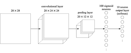
在这个架构中，我们可以把卷积和混合层看作是在学习输⼊训练图像中的局部感受野，而后面的全连接层则在⼀个更抽象的层次学习，从整个图像整合全局信息。这是⼀种常见的卷积神经网络模式。

在python解释器中输入下列代码：

>>> net = Network([
ConvPoolLayer(image_shape=(mini_batch_size, 1, 28, 28),
filter_shape=(20, 1, 5, 5),
poolsize=(2, 2)),
FullyConnectedLayer(n_in=20*12*12, n_out=100),
SoftmaxLayer(n_in=100, n_out=10)], mini_batch_size)
>>> net.SGD(training_data, 60, mini_batch_size, 0.1,
validation_data, test_data)

最终达到的准确率在98.78%左右，相比之前已经得到了很大的改善。

两层卷积网络

我们试着插⼊第二个卷积–混合层。把它插在已有的卷积–混合层和全连接隐藏层之间。我们再次使用⼀个 5 × 5 局部感受野，混合 2 × 2 的区域。

>>> net = Network([
        ConvPoolLayer(image_shape=(mini_batch_size, 1, 28, 28), 
                      filter_shape=(20, 1, 5, 5), 
                      poolsize=(2, 2)),
        ConvPoolLayer(image_shape=(mini_batch_size, 20, 12, 12), 
                      filter_shape=(40, 20, 5, 5), 
                      poolsize=(2, 2)),
        FullyConnectedLayer(n_in=40*4*4, n_out=100),
        SoftmaxLayer(n_in=100, n_out=10)], mini_batch_size)
>>> net.SGD(training_data, 60, mini_batch_size, 0.1, 
            validation_data, test_data) 

这一次我们的准确率可以达到99.06%。

修正线性单元

但是我们仍然可以通过改进我们的神经网络获得更好的分辨率。

这次我们使用修正线性单元，而不是S型激活函数。其表达式形式为:

f(z) ≡ max(0, z)。

关于修正线性单元的信息可以参考我之前的博客：改善神经网络学习的方法。

同时我们加入L2规范化，规范化参数λ = 0.1。

>>> from network3 import ReLU
>>> net = Network([
ConvPoolLayer(image_shape=(mini_batch_size, 1, 28, 28),
filter_shape=(20, 1, 5, 5),
poolsize=(2, 2),
activation_fn=ReLU),
ConvPoolLayer(image_shape=(mini_batch_size, 20, 12, 12),
filter_shape=(40, 20, 5, 5),
poolsize=(2, 2),
activation_fn=ReLU),
FullyConnectedLayer(n_in=40*4*4, n_out=100, activation_fn=ReLU),
SoftmaxLayer(n_in=100, n_out=10)], mini_batch_size)
>>> net.SGD(training_data, 60, mini_batch_size, 0.03,
validation_data, test_data, lmbda=0.1)

此时得到的分辨率应该为99.23%左右，相比之前又有了很大的提高。

拓展训练数据

在上面的基础上，我们以算法的形式拓展训练数据。

具体做法是将图像平移若干个像素，即可以得到一副新的图像。

我们在shell提示符中运行程序expend_mnist.py来实现数据的拓展。

$ python expend_mnist.py

运⾏这个程序取得 50, 000 幅 MNIST 训练图像并扩展为具有 250, 000 幅训练图像的训练集。然后我们可以使⽤这些训练图像来训练我们的网络。

>>> expanded_training_data, _, _ = network3.load_data_shared(
"../data/mnist_expanded.pkl.gz")
>>> net = Network([
ConvPoolLayer(image_shape=(mini_batch_size, 1, 28, 28),
filter_shape=(20, 1, 5, 5),
poolsize=(2, 2),
activation_fn=ReLU),
ConvPoolLayer(image_shape=(mini_batch_size, 20, 12, 12),
filter_shape=(40, 20, 5, 5),
poolsize=(2, 2),
activation_fn=ReLU),
FullyConnectedLayer(n_in=40*4*4, n_out=100, activation_fn=ReLU),
SoftmaxLayer(n_in=100, n_out=10)], mini_batch_size)
>>> net.SGD(expanded_training_data, 60, mini_batch_size, 0.03,
validation_data, test_data, lmbda=0.1)

最终可以得到99.37%左右的分辨准确率。

使用弃权的全连接层

在以上方法的基础上，我们再加一层全连接层，这样我们就有两个含有100个神经元的全连接层。

同时，将之前接触过的弃权技术运用到最终的全连接层上。

我们知道，弃权技术的基本思想是，在训练网络时随机的移除单独的激活值，降低网络的依赖性，有助于减轻过度拟合现象。参考博客：改善神经网络学习的方法。

>>> net = Network([
        ConvPoolLayer(image_shape=(mini_batch_size, 1, 28, 28), 
                      filter_shape=(20, 1, 5, 5), 
                      poolsize=(2, 2), 
                      activation_fn=ReLU),
        ConvPoolLayer(image_shape=(mini_batch_size, 20, 12, 12), 
                      filter_shape=(40, 20, 5, 5), 
                      poolsize=(2, 2), 
                      activation_fn=ReLU),
        FullyConnectedLayer(
            n_in=40*4*4, n_out=1000, activation_fn=ReLU, p_dropout=0.5),
        FullyConnectedLayer(
            n_in=1000, n_out=1000, activation_fn=ReLU, p_dropout=0.5),
        SoftmaxLayer(n_in=1000, n_out=10, p_dropout=0.5)], 
        mini_batch_size)
>>> net.SGD(expanded_training_data, 40, mini_batch_size, 0.03, 
            validation_data, test_data)

使用弃权的全连接层，我们的神经网络的分辨率提高到了99.60%。

使用组合网络

借助上面的方法，我们可以将准确率提高到99.60%左右。

⼀个简单的进⼀步提⾼性能的⽅法是创建几个神经网络，然后让它们投票来决定最好的分类。例如，假设我们使⽤上述的方式训练了 5 个不同的神经⽹络，每个达到了接近于 99.60% 的准确率。尽管网络都会有相似的准确率，他们很可能因为不同的随机初始化产生不同的错误。在这 5 个网络中进行⼀次投票来取得⼀个优于单个网络的分类，能进一步提高准确率。

源代码

以下是修改过的源代码，运行环境：python2.7，需要的库：numpy、theano

"""network3.py
~~~~~~~~~~~~~~

A Theano-based program for training and running simple neural
networks.

Supports several layer types (fully connected, convolutional, max
pooling, softmax), and activation functions (sigmoid, tanh, and
rectified linear units, with more easily added).

When run on a CPU, this program is much faster than network.py and
network2.py.  However, unlike network.py and network2.py it can also
be run on a GPU, which makes it faster still.

Because the code is based on Theano, the code is different in many
ways from network.py and network2.py.  However, where possible I have
tried to maintain consistency with the earlier programs.  In
particular, the API is similar to network2.py.  Note that I have
focused on making the code simple, easily readable, and easily
modifiable.  It is not optimized, and omits many desirable features.

This program incorporates ideas from the Theano documentation on
convolutional neural nets (notably,
http://deeplearning.net/tutorial/lenet.html ), from Misha Denil's
implementation of dropout (https://github.com/mdenil/dropout ), and
from Chris Olah (http://colah.github.io ).

Written for Theano 0.6 and 0.7, needs some changes for more recent
versions of Theano.

"""

#### Libraries
# Standard library
import cPickle
import gzip

# Third-party libraries
import numpy as np
import theano
import theano.tensor as T
from theano.tensor.nnet import conv
from theano.tensor.nnet import softmax
from theano.tensor import shared_randomstreams
#from theano.tensor.signal import downsample
from theano.tensor.signal import pool

# Activation functions for neurons
def linear(z): return z
def ReLU(z): return T.maximum(0.0, z)
from theano.tensor.nnet import sigmoid
from theano.tensor import tanh


#### Constants
GPU = True
if GPU:
    print "Trying to run under a GPU.  If this is not desired, then modify "+\
        "network3.py\nto set the GPU flag to False."
    try: theano.config.device = 'gpu'
    except: pass # it's already set
    theano.config.floatX = 'float32'
else:
    print "Running with a CPU.  If this is not desired, then the modify "+\
        "network3.py to set\nthe GPU flag to True."

#### Load the MNIST data
def load_data_shared(filename="../data/mnist.pkl.gz"):
    f = gzip.open(filename, 'rb')
    training_data, validation_data, test_data = cPickle.load(f)
    f.close()
    def shared(data):
        """Place the data into shared variables.  This allows Theano to copy
        the data to the GPU, if one is available.

        """
        shared_x = theano.shared(
            np.asarray(data[0], dtype=theano.config.floatX), borrow=True)
        shared_y = theano.shared(
            np.asarray(data[1], dtype=theano.config.floatX), borrow=True)
        return shared_x, T.cast(shared_y, "int32")
    return [shared(training_data), shared(validation_data), shared(test_data)]

#### Main class used to construct and train networks
class Network(object):

    def __init__(self, layers, mini_batch_size):
        """Takes a list of `layers`, describing the network architecture, and
        a value for the `mini_batch_size` to be used during training
        by stochastic gradient descent.

        """
        self.layers = layers
        self.mini_batch_size = mini_batch_size
        self.params = [param for layer in self.layers for param in layer.params]
        self.x = T.matrix("x")
        self.y = T.ivector("y")
        init_layer = self.layers[0]
        init_layer.set_inpt(self.x, self.x, self.mini_batch_size)
        for j in xrange(1, len(self.layers)):
            prev_layer, layer  = self.layers[j-1], self.layers[j]
            layer.set_inpt(
                prev_layer.output, prev_layer.output_dropout, self.mini_batch_size)
        self.output = self.layers[-1].output
        self.output_dropout = self.layers[-1].output_dropout

    def SGD(self, training_data, epochs, mini_batch_size, eta,
            validation_data, test_data, lmbda=0.0):
        """Train the network using mini-batch stochastic gradient descent."""
        training_x, training_y = training_data
        validation_x, validation_y = validation_data
        test_x, test_y = test_data

        # compute number of minibatches for training, validation and testing
        num_training_batches = size(training_data)/mini_batch_size
        num_validation_batches = size(validation_data)/mini_batch_size
        num_test_batches = size(test_data)/mini_batch_size

        # define the (regularized) cost function, symbolic gradients, and updates
        l2_norm_squared = sum([(layer.w**2).sum() for layer in self.layers])
        cost = self.layers[-1].cost(self)+\
               0.5*lmbda*l2_norm_squared/num_training_batches
        grads = T.grad(cost, self.params)
        updates = [(param, param-eta*grad)
                   for param, grad in zip(self.params, grads)]

        # define functions to train a mini-batch, and to compute the
        # accuracy in validation and test mini-batches.
        i = T.lscalar() # mini-batch index
        train_mb = theano.function(
            [i], cost, updates=updates,
            givens={
                self.x:
                training_x[i*self.mini_batch_size: (i+1)*self.mini_batch_size],
                self.y:
                training_y[i*self.mini_batch_size: (i+1)*self.mini_batch_size]
            })
        validate_mb_accuracy = theano.function(
            [i], self.layers[-1].accuracy(self.y),
            givens={
                self.x:
                validation_x[i*self.mini_batch_size: (i+1)*self.mini_batch_size],
                self.y:
                validation_y[i*self.mini_batch_size: (i+1)*self.mini_batch_size]
            })
        test_mb_accuracy = theano.function(
            [i], self.layers[-1].accuracy(self.y),
            givens={
                self.x:
                test_x[i*self.mini_batch_size: (i+1)*self.mini_batch_size],
                self.y:
                test_y[i*self.mini_batch_size: (i+1)*self.mini_batch_size]
            })
        self.test_mb_predictions = theano.function(
            [i], self.layers[-1].y_out,
            givens={
                self.x:
                test_x[i*self.mini_batch_size: (i+1)*self.mini_batch_size]
            })
        # Do the actual training
        best_validation_accuracy = 0.0
        for epoch in xrange(epochs):
            for minibatch_index in xrange(num_training_batches):
                iteration = num_training_batches*epoch+minibatch_index
                if iteration % 1000 == 0:
                    print("Training mini-batch number {0}".format(iteration))
                cost_ij = train_mb(minibatch_index)
                if (iteration+1) % num_training_batches == 0:
                    validation_accuracy = np.mean(
                        [validate_mb_accuracy(j) for j in xrange(num_validation_batches)])
                    print("Epoch {0}: validation accuracy {1:.2%}".format(
                        epoch, validation_accuracy))
                    if validation_accuracy >= best_validation_accuracy:
                        print("This is the best validation accuracy to date.")
                        best_validation_accuracy = validation_accuracy
                        best_iteration = iteration
                        if test_data:
                            test_accuracy = np.mean(
                                [test_mb_accuracy(j) for j in xrange(num_test_batches)])
                            print('The corresponding test accuracy is {0:.2%}'.format(
                                test_accuracy))
        print("Finished training network.")
        print("Best validation accuracy of {0:.2%} obtained at iteration {1}".format(
            best_validation_accuracy, best_iteration))
        print("Corresponding test accuracy of {0:.2%}".format(test_accuracy))

#### Define layer types

class ConvPoolLayer(object):
    """Used to create a combination of a convolutional and a max-pooling
    layer.  A more sophisticated implementation would separate the
    two, but for our purposes we'll always use them together, and it
    simplifies the code, so it makes sense to combine them.

    """

    def __init__(self, filter_shape, image_shape, poolsize=(2, 2),
                 activation_fn=sigmoid):
        """`filter_shape` is a tuple of length 4, whose entries are the number
        of filters, the number of input feature maps, the filter height, and the
        filter width.

        `image_shape` is a tuple of length 4, whose entries are the
        mini-batch size, the number of input feature maps, the image
        height, and the image width.

        `poolsize` is a tuple of length 2, whose entries are the y and
        x pooling sizes.

        """
        self.filter_shape = filter_shape
        self.image_shape = image_shape
        self.poolsize = poolsize
        self.activation_fn=activation_fn
        # initialize weights and biases
        n_out = (filter_shape[0]*np.prod(filter_shape[2:])/np.prod(poolsize))
        self.w = theano.shared(
            np.asarray(
                np.random.normal(loc=0, scale=np.sqrt(1.0/n_out), size=filter_shape),
                dtype=theano.config.floatX),
            borrow=True)
        self.b = theano.shared(
            np.asarray(
                np.random.normal(loc=0, scale=1.0, size=(filter_shape[0],)),
                dtype=theano.config.floatX),
            borrow=True)
        self.params = [self.w, self.b]

    def set_inpt(self, inpt, inpt_dropout, mini_batch_size):
        self.inpt = inpt.reshape(self.image_shape)
        conv_out = conv.conv2d(
            input=self.inpt, filters=self.w, filter_shape=self.filter_shape,
            image_shape=self.image_shape)
        pooled_out = pool.pool_2d(
            input=conv_out, ws=self.poolsize, ignore_border=True)
        self.output = self.activation_fn(
            pooled_out + self.b.dimshuffle('x', 0, 'x', 'x'))
        self.output_dropout = self.output # no dropout in the convolutional layers

class FullyConnectedLayer(object):

    def __init__(self, n_in, n_out, activation_fn=sigmoid, p_dropout=0.0):
        self.n_in = n_in
        self.n_out = n_out
        self.activation_fn = activation_fn
        self.p_dropout = p_dropout
        # Initialize weights and biases
        self.w = theano.shared(
            np.asarray(
                np.random.normal(
                    loc=0.0, scale=np.sqrt(1.0/n_out), size=(n_in, n_out)),
                dtype=theano.config.floatX),
            name='w', borrow=True)
        self.b = theano.shared(
            np.asarray(np.random.normal(loc=0.0, scale=1.0, size=(n_out,)),
                       dtype=theano.config.floatX),
            name='b', borrow=True)
        self.params = [self.w, self.b]

    def set_inpt(self, inpt, inpt_dropout, mini_batch_size):
        self.inpt = inpt.reshape((mini_batch_size, self.n_in))
        self.output = self.activation_fn(
            (1-self.p_dropout)*T.dot(self.inpt, self.w) + self.b)
        self.y_out = T.argmax(self.output, axis=1)
        self.inpt_dropout = dropout_layer(
            inpt_dropout.reshape((mini_batch_size, self.n_in)), self.p_dropout)
        self.output_dropout = self.activation_fn(
            T.dot(self.inpt_dropout, self.w) + self.b)

    def accuracy(self, y):
        "Return the accuracy for the mini-batch."
        return T.mean(T.eq(y, self.y_out))

class SoftmaxLayer(object):

    def __init__(self, n_in, n_out, p_dropout=0.0):
        self.n_in = n_in
        self.n_out = n_out
        self.p_dropout = p_dropout
        # Initialize weights and biases
        self.w = theano.shared(
            np.zeros((n_in, n_out), dtype=theano.config.floatX),
            name='w', borrow=True)
        self.b = theano.shared(
            np.zeros((n_out,), dtype=theano.config.floatX),
            name='b', borrow=True)
        self.params = [self.w, self.b]

    def set_inpt(self, inpt, inpt_dropout, mini_batch_size):
        self.inpt = inpt.reshape((mini_batch_size, self.n_in))
        self.output = softmax((1-self.p_dropout)*T.dot(self.inpt, self.w) + self.b)
        self.y_out = T.argmax(self.output, axis=1)
        self.inpt_dropout = dropout_layer(
            inpt_dropout.reshape((mini_batch_size, self.n_in)), self.p_dropout)
        self.output_dropout = softmax(T.dot(self.inpt_dropout, self.w) + self.b)

    def cost(self, net):
        "Return the log-likelihood cost."
        return -T.mean(T.log(self.output_dropout)[T.arange(net.y.shape[0]), net.y])

    def accuracy(self, y):
        "Return the accuracy for the mini-batch."
        return T.mean(T.eq(y, self.y_out))


#### Miscellanea
def size(data):
    "Return the size of the dataset `data`."
    return data[0].get_value(borrow=True).shape[0]

def dropout_layer(layer, p_dropout):
    srng = shared_randomstreams.RandomStreams(
        np.random.RandomState(0).randint(999999))
    mask = srng.binomial(n=1, p=1-p_dropout, size=layer.shape)
    return layer*T.cast(mask, theano.config.floatX)