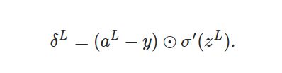
classNetwork(object): ... """backprop函数实现反向传播算法""" defbackprop(self, x, y): """Return a tuple "(nabla_b, nabla_w)" representing the gradient for the cost function C_x. "nabla_b" and "nabla_w" are layer-by-layer lists of numpy arrays, similar to "self.biases" and "self.weights".""" #初始化b,w的偏导数,得到相应的结构,数值均为0 nabla_b = [np.zeros(b.shape) for b in self.biases] nabla_w = [np.zeros(w.shape) for w in self.weights] # feedforward #第一层的激活值等于输入值 activation = x activations = [x] # list to store all the activations, layer by layer zs = [] # list to store all the z vectors, layer by layer #依次计算每层的带权输入和激活值 for b, w in zip(self.biases, self.weights): z = np.dot(w, activation)+b zs.append(z) activation = sigmoid(z) activations.append(activation) # backward pass #输出层误差delta delta = self.cost_derivative(activations[-1], y) * \ sigmoid_prime(zs[-1]) #使用公式BP3和BP4,由误差得到b和w的偏导 nabla_b[-1] = delta nabla_w[-1] = np.dot(delta, activations[-2].transpose()) # Note that the variable l in the loop below is used a little # differently to the notation in Chapter 2 of the book. Here, # l = 1 means the last layer of neurons, l = 2 is the # second-last layer, and so on. It's a renumbering of the # scheme in the book, used here to take advantage of the fact # that Python can use negative indices in lists. #反向传播,得到每一层的误差,再得到每一层的偏导 for l in xrange(2, self.num_layers): z = zs[-l] sp = sigmoid_prime(z) delta = np.dot(self.weights[-l+1].transpose(), delta) * sp nabla_b[-l] = delta nabla_w[-l] = np.dot(delta, activations[-l-1].transpose()) #返回本次迭代得到的b和w return (nabla_b, nabla_w)
... #二次代价函数对激活值a求导 defcost_derivative(self, output_activations, y): """Return the vector of partial derivatives \partial C_x / \partial a for the output activations.""" return (output_activations-y) #z型神经元的输出函数 defsigmoid(z): """The sigmoid function.""" return1.0/(1.0+np.exp(-z)) #输出函数的导数 defsigmoid_prime(z): """Derivative of the sigmoid function.""" return sigmoid(z)*(1-sigmoid(z))